On this page you can learn more about:
- Integrity Monitoring
- Navigation System Theory
- Integrated Navigation Systems
- Navigation System Theory
- Fault-tolerant Navigation Systems
Integrity Monitoring
Certification rules for safety-critical applications require availability of a fault-free navigation solution, that probability of failing to identify a fault is low and a fault is detected sufficiently fast. Tasks of fault detection, protection of navigation solution from corruption and verification of its consistency are called altogether integrity monitoring.
Fault detection (FD) usually means that user is only informed about fault occurrence. Fault detection and recovery (FDR) supposes that error source is identified and navigation solution is attempted to be recovered from corruption caused by the fault. Fault detection and isolation (FDI) means capability to provide uncontaminated navigation solution.
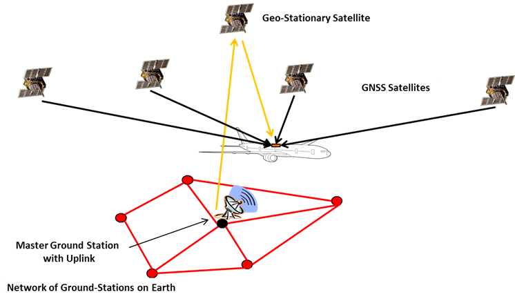
Integrity monitoring techniques can be divided into two classes: sensor-level (user-based) techniques and system-level (infrastructure-based) techniques. The most well-known sensor-level approaches are range checks, Kalman filer innovation monitoring, consistency checks of quantities calculated from different combinations of measurements. In radio navigation systems transmitted signal errors can more easily be detected by monitoring stations rather than by an user receiver.
Where monitoring infrastructure is acceptable to be used and available, system-level integrity monitoring is preferable.
Literature
- P. D. Groves, Principles of GNSS, inertial, and multisensor integrated navigation systems, 2nd ed. Boston, Mass.: Artech House, 2013.
Navigation System Theory
Navigation system theory mainly deals with stability, observability and controllability.
Stability theory investigates the nature of the propagation of navigation states initialization errors. The stability properties of inertial navigation are borderline in the sense that most combinations of navigation state initialization errors neither decay nor amplify. Due to the central gravity field just two combinations behave different. The so-called vertical channel as a linear combination of vertical position and vertical velocity error components is exponentially instable, i.e. grow with an exponential amplification factor.
In contrast the so-called horizontal channel is periodic with a Schuler period of about 84 minutes on topographic level. Of course inertial sensor errors cause a navigation solution divergence on top of these effects.
Observability theory searches for answers on how good the navigation states can be deduced when knowing the system inputs (inertial sensor measurements) and system outputs (navigation observations) together with at least some of their time derivatives. The observability properties do obviously depend upon the underlying trajectory. Well known is the lack of observability of North-indicating heading in straight and levelled flight. Generally speaking in all flight situations the angle around the currently measured acceleration vector is in general not observable.
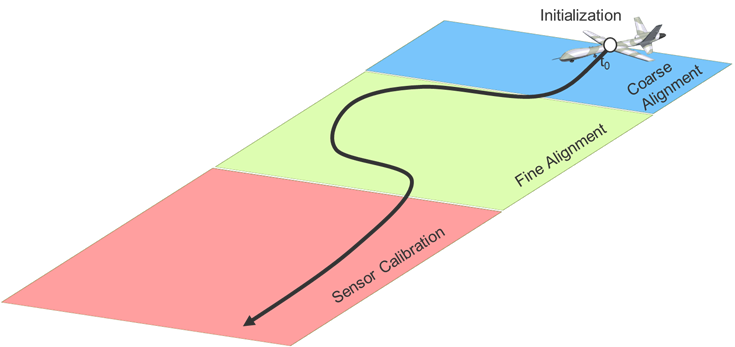
Especially when adding bias-like sensor, model and observation errors to the basic navigation errors states the observability gets difficult to assess, since the number of unknowns grow, whereas the number of observations remains low. Thus the observability of individual states is derived through manoeuvre changes.
The alignment manoeuvre of fighter aircraft pilots for the effector fine alignment is a prominent example for this interrelation.
Literature
- Seminar “Navigation and Data Fusion”.
- I. Y. Bar-Itzhack and B. Porat, “Azimuth Observability Enhancement During Inertial Navigation In-Flight Alignment,” Guidance and Control, vol. 3, no. 4, pp. 337–344, 1980.
- A. Dachs, “Rechenzeitoptimierung, Robustifizierung und Tuning eines Kalmanfilters zur Datenfusion für Navigationsanwendungen,” Schriftenreihe Geoinformationsdienst der Bundeswehr, no. 3, 2010.
- J. Dambeck, Diagnose und Therapie geodätischer Trägheitsnavigationssysteme. Dissertation: Universität Stuttgart, 1998.
- R. Hermann and A. J. Krener, “Nonlinear Controllability and Observability,” IEEE Transactions on Automatic Control, vol. 22, no. 5, pp. 728–740, 1977.
Integrated Navigation Systems
Inertial navigation provides six degrees of freedom, i.e. three translational and three rotational, and an inherently high update rate, but is just short to medium term stable due to timely integration of initialization, inertial sensor measurement and gravity model errors.
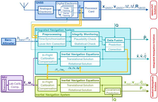
On the other hand satellite navigation performs long term stable positioning at a comparatively low update rate. Thus both navigation approaches provide complementary properties in a somewhat ideal way. When GNSS position and (Doppler) velocity are used to aid inertial navigation the underlying IMU/GNSS integration architecture is called loosely-coupled, since for an unfiltered GNSS (position, velocity and time) solution at least lock to four satellites is required.
An IMU/GNSS integration architecture is called tightly-coupled if pseudo- and delta ranges to each satellite are used instead. In a deeply-integrated IMU/GNSS integration the correlation inside the GNSS receiver is controlled from the outside to aim for a centralized filter architecture. Whereas inertial navigation does not depend upon transmission or reception of any signals, satellite navigation does with an inherently low signal strength quite below background noise. Antenna shading by manoeuvres, terrain shading or signal interference may cause availability outages depending on satellite constellation, application and anthropogenic disturbances.
Due to the instability of the (inertial) vertical translational channel mainly caused by the central gravity field an permanently available vertical aiding is commonly used. In flight navigation applications usually the barometric altitude derived from static pressure is used, relative to which airplanes are vertically separated. In marine applications typically zero height aiding is applied.
This approach typically describes the situation when using navigation grade inertial sensors, where position accuracies in the order of nautical miles per hour are achieved. Size, weight, power, detailed design and moding depend upon the underlying application.
Literature
- Seminar “Navigation and Data Fusion”.
- D. J. Biezad, Integrated navigation and guidance systems. Reston, Va.: American Institute of Aeronautics and Astronautics, 1999.
- J. L. Farrell, Integrated aircraft navigation, 9th ed. San Diege: Academic Press, 1994.
- P. D. Groves, Principles of GNSS, inertial, and multisensor integrated navigation systems, 2nd ed. Boston, Mass.: Artech House, 2013.
- R. M. Rogers, Applied mathematics in integrated navigation systems, 2nd ed. Reston, Va.: American Institute of Aeronautics and Astronautics, 2003.
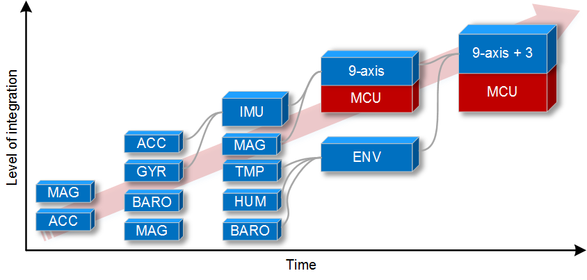
Lost-Cost MEMS Combo Navigation Systems
MEMS sensors dominate the market due to size, weight, power and cost (SWaP-C) constraints in many applications.
Low-cost MEMS IMUs typically have a poor turn-on bias repeatability and large sensor noise. The turn-on bias shows a statistical behaviour for a large ensemble of repetitions, but is bias-like for a single mission. Thus the turn-on MEMS IMU biases must be quickly estimated in-motion. Nevertheless the inertial MEMS sensor errors will cause a fast kinematic state divergence and thus require more or less permanent aiding of all six degrees of freedom.
Since GNSS denied environments cannot be avoided in many applications, operation without GNSS receiver shall be possible. Therefore the rotational three degrees of freedom are typically aided by accelerometer and magnetometer measurements. The translational equations of motion can in general be separated into the vertical and horizontal channels. The vertical channel can be aided by barometric altitude from static pressure measurements. The horizontal channel for flight applications can either be aided using airdata like true airspeed (TAS), angle of attack (AOA) and angle of sideslip (AOS), aerodynamic model or by camera vision. Land applications will use odometry and vehicle driving dynamics instead. (Sub-)Marine applications use log speed and vessel hydrodynamics.
The large bias-like sensor errors require filter state vector augmentation for their estimation on the one and nonlinear filtering on the other hand, whereas large noise-like sensor errors require high filter frequencies on the one and computational filter efficiency on the other hand. Thus low-cost navigation applications in many situations will be mathematically more demanding than classical high-precision navigation.
Fault-Tolerant Navigation Systems
Every year automatically controlled vehicles get more and more involved into humans daily activities.
That is why safety of life very often depends either explicitly or implicitly on proper operation of control unit which in its turn cannot function without reliable navigational solution. Consequently development of fault-tolerant navigation systems becomes highly important.

Primary task of any fault-tolerant system is to detect failure, isolate the component responsible for it (Fault Detection and Isolation, FDI), monitor system integrity and emit an alarm if the output cannot be trusted. Classical FDI algorithms are based on Generalized Likelihood Ratio Test method and parity space approach. However recently new methods based on Mahalanobis distance have been developed to improve performance of low-cost architectures.
Integrity of a system can be characterized by such parameters as Time to Alert (TTA) and Alert Limits. TTA is the maximum allowable time elapsed from onset of system being out of tolerance until equipment enunciates the alert. Alert Limit for a given parameter measurement is the error tolerance not to be exceeded without issuing an alert.
Each system malfunction may cause different consequences. Failure mode and effect analysis (FMEA) is a systematic technique which is intended to study possible faults, their causes and outcomes. Numerous performance tests are prescribed by certification authorities to assure that probable malfunctions can happen infrequently and that in case of an actual failure cabin crew gets adequate warning.
Literature
- P. D. Groves, Principles of GNSS, inertial, and multisensor integrated navigation systems, 2nd ed. Boston, Mass.: Artech House, 2013.
- International Civil Aviation Organization, To The Convention On International Civil Aviation, Volume I – Radio Navigation Aids, International Standards And Recommended Practices (SARPs), Doc. AN10-1, 2006.
| ⇦ Data Fusion | return to overview | Laboratory Testing⇨ |