On this page you can learn more about:
- Earth’s Gravity Field
- Earth’s Magnetic Field
- Digital Surface Model
- Bearings
- Spherical Positioning
- Hyperbolic Positioning
Earth’s Gravity Field
Physical geodesy is the classical theory of the gravity field of the Earth as superposition of the gravitation and centrifugal fields.
Cartesian, spherical, geodetic and ellipsoidal coordinates are alternatively used. The gravitation field of the Earth can be either described in integral or differential form. Since the (simpler) integral form requires sufficient knowledge of the mass density distribution inside the Earth, commonly the differential formulation just requiring boundary information is used. A mathematical theory called potential (field) theory constitutes the mathematical background. The gravitational potential field outside masses fulfills the so-called Laplace partial differential equation. Searching for a solution for an (almost) spherical body, the Laplace partial differential equation is transformed into spherical coordinates and then solved by the method of separation of variables. Three ordinary differential equations are derived in this way, which solutions are known. Combining these solutions to solid spherical harmonics the gravitation potential field can be described in a superposition of decaying spherical oscillations in a similar way as is known from Fourier theory on a circle. The coefficients have been identified from geodetic field measurements and satellite missions.
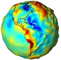
The commonly used set of coefficients is called Earth Gravity Model 2008 (EGM2008) and is integral part of the World Geodetic System 1984 (WGS84). The gravitation potential field of a homogeneous ellipsoid of revolution can be solved in closed-form using ellipsoidal coordinates. From this formulation the normal gravity formula of Somigliana was derived on the equipotential ellipsoid and extended around it by a Taylor series expansion called free air reduction. The gravity vector field, as gradient of the gravity potential field is sufficient and commonly used in less accurate navigation applications. Experiencing stronger variations of the gravity field, e.g. along the fringe of the Alps, or when precise accelerometers are used, more accurate Earth’s gravity field modelling is required.
Literature
- Seminar “Navigation and Data Fusion”.
- National Imagery and Mapping Agency (NIMA), World Geodetic System 1984, Its Definition and Relationships with Local Geodetic Systems: Amendment 1, 3rd ed, 2000.
- S. Chandrasekhar, Ellipsoidal figures of equilibrium. New York: Dover, 1987.
- W. A. Heiskanen and H. Moritz, Physical geodesy. San Francisco: Freeman, 1967.
- H. Moritz, The figure of the earth: Theoretical geodesy and the earth’s interior. Karlsruhe: Wichmann, 1990.
- N. N. Lebedev and R. A. Silverman, Special functions and their applications. Englewood Cliffs, N.J.: Prentice-Hall, 1965.
Earth’s Magnetic Field
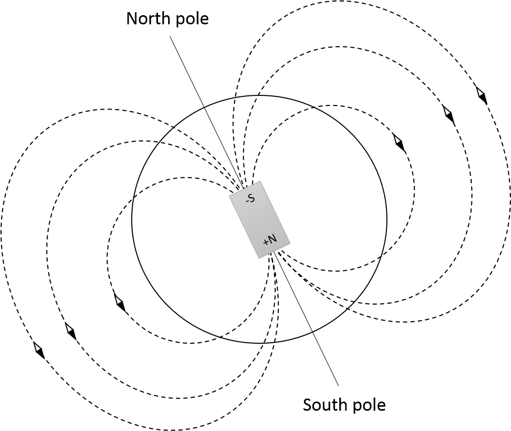
The earth magnetic field vector provides a valuable navigation reference as long as disturbances by other magnetic fields are small. E.g. in high altitudes, measurements agree closely with mathematical models and a vector observation can be used to derive orientation of measurement axes (with one remaining degree of unknown rotation).
The simplest model of Earth’s magnetic field is a tilted dipole located near the center of the Earth. This model is very rough but allows to understand basic properties of the measurement and to estimate its usability for different applications. World Magnetic Model (WMM) and Enhanced Magnetic Model (EMM) are high-fidelity empirical models of Earth’s magnetic field. WMM uses spherical harmonics representation to degree and order 12 and resolves magnetic field at 3000 km wavelength. EMM extends to degree and order 720 and resolves magnetic anomalies down to 56 km wavelength.
Unlike gravity, which can only be measured during straight and leveled flight, magnetic field measurement is independent of flight parameters and hence presents a more robust source of information on vehicle’s attitude.
Literature
- W. J. Hinze, Von Frese, Ralph R. B, and A. H. Saad, Gravity and magnetic exploration: Principles, practices and applications. Cambridge: Cambridge University Press, 2013.
- S. Maus, S. Macmillan, and S. McLean, The US/UK World Magnetic Model for 2015-2020. Boulder, CO, Edinburgh: NOAA National Geophysical Data Center; British Geological Survey Geomagnetism Team, 2015.
- S. Maus, “An ellipsoidal harmonic representation of Earth’s lithospheric magnetic field to degree and order 720,” Geochemistry, Geophysics, Geosystems, vol. 11, 2010.
Digital Surface Model
Formerly Digital Terrain Models (DTM) have been obtained by digitalizing topographic maps. The collection and digitalization of maps turned out to be a never-ending task with nevertheless low possibility to cover the about 150 million square-kilometers of the Earth’s land masses sufficiently.
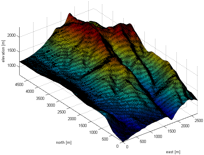
With the advent of remote sensing from space the coverage improved, but due to satellite mission limitations, satellite maintenance maneuvers, bad radar reflections (either caused by too steep signal impact angles or low reflectivity) or a non-polar satellite orbit the coverage by just a singular satellite mission was not sufficient, e.g. Shuttle Radar Topography Mission (SRTM). Therefore the reflected radar signals of several satellite missions have been jointly processed in order to achieve a quality-controlled DSM. Later the orbits became polar in order to achieve full coverage of the Earth. Today the two German satellites TerraSAR-X and TanDEM-X are in formation orbiting the Earth in order to collect sufficient signals for a full coverage of the Earth in so far unparalleled coverage and resolution. The resulting DSM is called WorldDEM and comes with resolutions as high as 0,4 arcsec or 12m in equatorial regions. Due to polar convergence the angular resolution in east-west-direction gets coarser with higher latitudes. Beside the actual surface heights also an accuracy layer is computed, such that the more from the less accurate surface areas can be distinguished, which is of utmost interest for terrain- or surface-following operations, respectively.
A typical format the DSM is provided in is called Digital Terrain Elevation Data (DTED), which is a bit misleading, but the term has been retained from its roots in DTMs. All kinds of surface ranging sensors require a sufficiently good DSM. In case of surface range-imaging sensors either georeferenced and orthorectified satellite images projected onto a DSM or 3D maps are needed.
Literature
- Kayton and W. R. Fried, Avionics navigation systems, 2nd ed. New York: Wiley, 1997.
- M. Siouris, Aerospace avionics systems: A modern synthesis. San Diego: Acad. Press, 1993.
- M. Siouris, Missile guidance and control systems. New York: Springer, 2004.
- M. Grey and R. S. Dale, “Recent Developments in TERPROM,” AGARD Conference Proceedings No. 455: Advances in Techniques and Technologies for Air Vehicle Navigation and Guidance, 1989.
- P. Golden, “Terrain Contour Matching (TERCOM): A cruise missile guidance aid,” SPIE Vol. 238 Image Processing for Missile Guidance, pp. 10–18, 1980.
- D. Andreas, L. D. Hostetler, and R. C. Beckmann, “Continuous Kalman Updating of an Inertial navigation System using Terrain Measurements,” Nat. Aerospace. Electronics Conference Proceedings, pp. 1263–1270, 1978.
Bearings
The usage of bearings is probably one of the oldest navigation technique. Basically, it is a method of describing the direction from ones current position towards an object’s position. Bearings can be given either relative to the current heading or to a reference direction. In early times this reference direction was mostly given by landmarks or celestial bodies. Today, mostly true north is used as a reference for surveying, while magnetic north is used in less demanding applications. Radionavigation presents some kind of advancement compared to classical bearing, as the landmarks are replaced by radio beacons that do not rely on optical visibility.
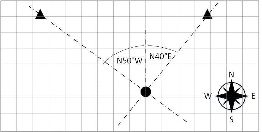
The determination of the current position requires the bearing and distance to a landmark or bearings towards at least two landmarks which are not on a straight line with the current location. The intersection of both bearings marks the current position. Using a bearing compass the bearing of an object relative to the magnetic north can be easily determined. Classically bearings are measured in degrees or mils. As a mil approximates the sinus of small angles, the use of mils simplifies the distance estimation for objects of a known size.
Literature
- Headquarters Department of the Army, Field Manual 3-25.26: Map Reading and Land Navigation. Washington D.C.
- G. Major, Quo vadis: Evolution of modern navigation: The rise of quantum techniques. New York u.a.: Springer, 2014.
Spherical Positioning
In general there are two ways of spherical positioning: unidirectional and bidirectional ranging by communication runtime measurements. In case of bidirectional ranging a user transceiver sends a signal to a repeater at a known location with no or an a priori known delay between reception and transmission. This concept allows on the one hand ranging without the need for a precise clock in the user receiver, but limits on the other hand the number of users per reference station.
In two dimensions ranging to two reference stations gives two solutions in the plane and in three dimensions ranging to three reference stations gives two solutions of which just one has in general the right altitude. In both cases ranging to another reference station sorts out the ambiguity. In case of unidirectional ranging a user receives the signal sent from reference stations.
To be able to measure range not just the reference stations but also the users have the need for precise synchronized clocks. When the requirements for the user receivers regarding a precise clock are relaxed just pseudoranges, as superpositions of ranges and receiver clock errors, are measured. This concept has been realized in satellite navigation to serve an arbitrary number of users simultaneously. Geometrically the user receiver clock error inflates simultaneously the spheres of possible locations around the reference stations.
In three dimensions pseudoranging to four reference stations is required to solve instantly for user position and receiver clock error. In case of known altitude just three pseudoranges are required to calculate the horizontal user location and the receiver clock error. In filtered pseudoranging solutions a coasting clock error estimate further relaxes the number of reference station to be used.
Literature
- Seminar “Navigation and Data Fusion”.
Hyperbolic Positioning
Unidirectional ranging without precise user receiver clocks results in pseudorange (runtime) measurements as superposition of range to reference station and receiver clock error.
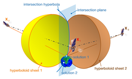
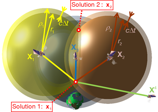
Differencing two pseudorange measurements cancels out the receiver clock error. In two dimensions the user is located along two hyperbolas with the reference stations in their foci. In three dimensions the user is located on a hyperboloid of two sheets with the reference stations (e.g. satellites) in their foci.
Pseudoranging to three reference stations allows two pseudorange differences corresponding to range differences. The reference station contained in both differences then is a focus point of both hyperboloids of two sheets. Confocal hyperboloid branches intersect in a plane hyperbola along which the user is located.
Intersecting the hyperbola with the Earth’s surface results in ambiguous solutions. Incorporating another space-time sphere, corresponding to a fourth pseudorange, again results in ambiguous solutions of which one should be extraterrestrial. Classical radionavigation systems, like LORAN-C, have been used for marine and flight applications. With the advent of satellite navigation most classical radionavigation systems have been overcome.
Differencing, like hyperbolic positioning, is commonly used in satellite navigation.
Literature
- J. Dambeck and B. Braun, “Analytical 2D GNSS PVT solutions from a hyperbolic positioning approach,” GPS Solutions, vol. 17, no. 3, pp. 309–326, 2013.
- B. Fang, “Simple Solutions for Hyperbolic and Related Position Fixes,” IEEE Transactions on Aerospace and Electronic Systems, vol. 26, pp. 748–753, 1990.
- A. Kleusberg, “Die direkte Lösung des Hyperbelschnitts,” Zeitschritt für Vermessungswesen, vol. 119, no. 4, pp. 188–192, 1994.
| ⇦ Certification and Export Regulations | return to overview | Inertial Navigation ⇨ |